How to Shape Model - Part 7 - Model visualization

In this tutorial, I’ll go over different strategies to visualize your shape model.

This is the seventh tutorial in the series on how to create statistical shape models. So far, we’ve only visualized our model through manual inspection in Scalismo-UI, but a number of additional useful visualization methods exist.

Shape Model GIF

If you are to include your model on a website or in a presentation, I often find it much more engaging to make a small animation of how the model deforms. A typical strategy I use is to write the principal components from 0 to 3 standard deviation, back to -3 and to 0, and do so for the top principal components. Before diving into the code, let’s look at the resulting animation that we are looking to represent:

The first step is to write meshes to a folder for each change to the model parameters. First, we define the values each component should take, i.e., from $0$ to $3.0$ to $0$ to $-3.0$ and to $0$. Depending on your model, it might make sense to only show $+/- 2.0$ or $+/- 1$ standard deviation as $3.0$ standard deviation is a very unlikely shape.

  val valstop = 30
  val stepSize = 5
  val rangeInts =
    (0 to valstop by stepSize) ++ (valstop to -valstop by -stepSize) ++ (-valstop to 0 by stepSize)
  val rangeDouble = rangeInts.map(f => f.toDouble / 10.0)

Next, we define the components that we want to capture, in this case, components 0, 1, and 2. Then, we create a function to write the steps to a folder

  val outputDir = new File("data/tmp/")

  def processComponent(comp: Int): Unit = {
    rangeDouble.foreach { v =>
      val modelPars = DenseVector.zeros[Double](ssm.rank)
      modelPars(comp) = v
      val instance = ssm.instance(modelPars)
      MeshIO.writeMesh(
        instance,
        new File(outputDir, s"${"ssm_%04d".format(cnt)}.ply")
      )
      cnt += 1
    }
  }

  val components = Seq(0, 1, 2)
  components.foreach { comp =>
    println(s"Component: $comp")
    processComponent(comp)
  }

The next step is to load the mesh sequence into Paraview. Select all the meshes from the output folder and drag them to the browser area in Paraview.

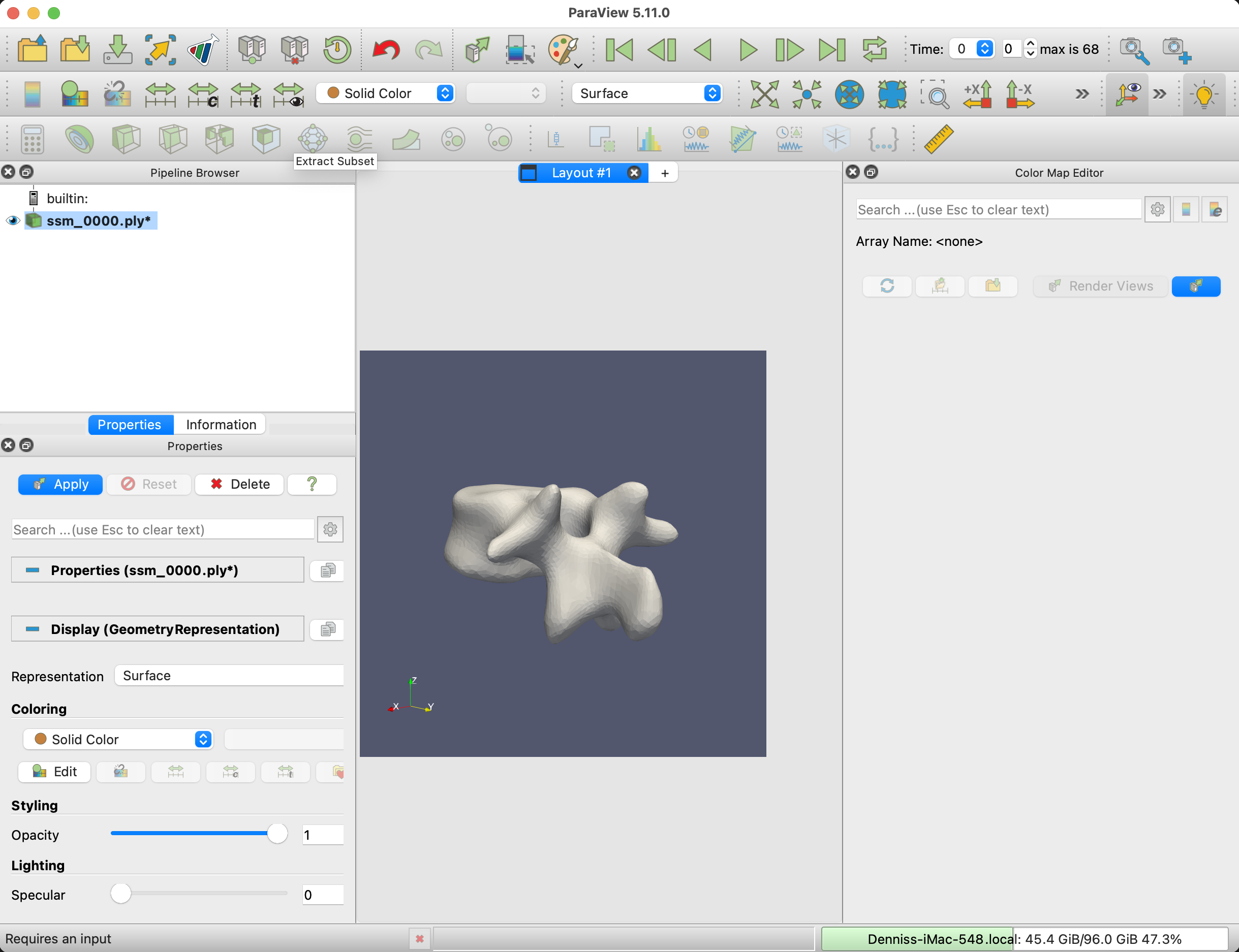
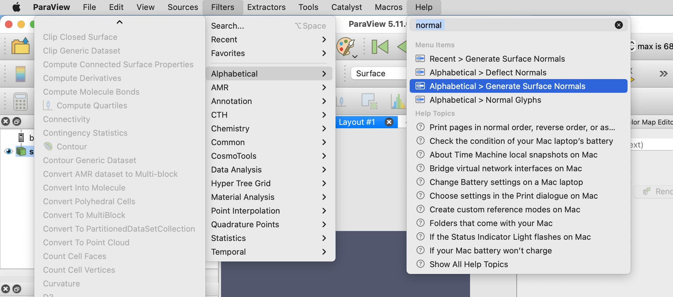
To smoothen the mesh visualization, apply the Generate Surface Normals filter to the mesh.

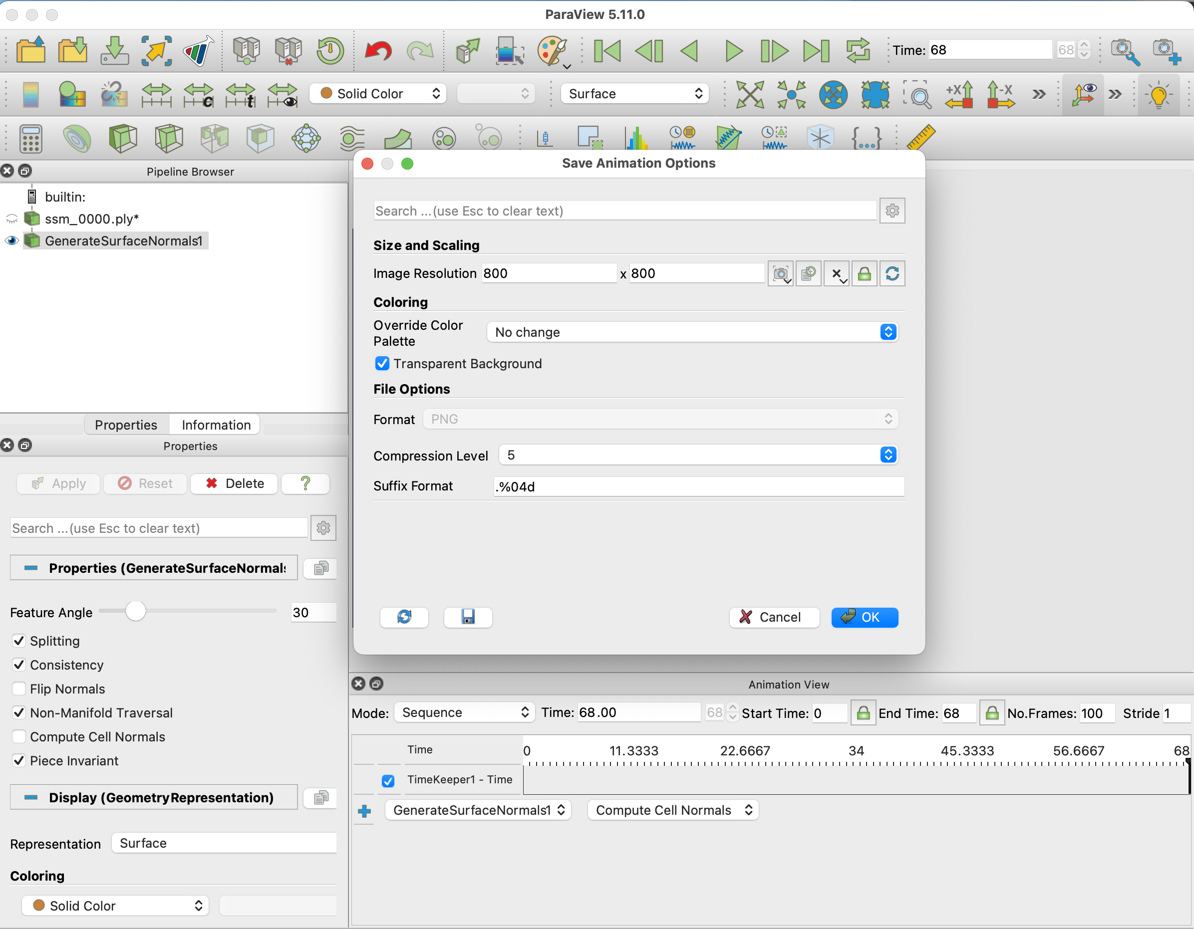
Next, set the canvas size to the dimensions that you would like the animation to be under View -> Preview -> Custom, in this example, I choose an image size of $800x800$ pixels.

If the Animation view is not visible, enable it view -> Animation View. Set Mode to Sequence, set the start time to $0$, the end time to the number of meshes in your exported folder, and the No. Frames to the frame rate times the animation duration. In our case, we chose 25FPS and the clip to last 4 seconds, which means 100 frames.

Using the Play button at the top, check how the animation looks like. And check that the mesh is positioned correctly in the scene.

The last step in Paraview is now to export the animation. I recommend exporting it as PNG files and converting those to a GIF afterward. Alternatively, Paraview also has a video export option. To export File -> Save Animation..., select a name, folder, and in the Animation Optionts, remember to choose Transparent Background.

Finally, we need to convert the PNG files to a GIF. This can be done using (Imagemagick)[https://imagemagick.org/index.php]. With the terminal, CD into the folder with the PNG files and execute

convert -delay 4 -loop 0 -alpha set -dispose previous *.png ssm.gif

This will create the final GIF file. NOTE that the -delay is in 100ths of a second, so 4 is 0.04 seconds, meaning a frame rate of 25 fps.

If the animation isn’t smooth enough, then go back and export a more dense set of meshes.

Correspondence Color

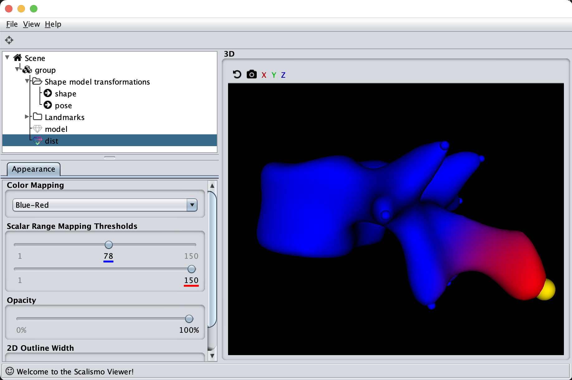
Another helpful visualization technique is to show the point correlation in the model. For this, we will select a point on the model and color the mesh based on the correlation with the selected point. This method is also good to use when manually defining the model kernels.

  val model: PointDistributionModel[_3D, TriangleMesh] = ??? 
  val lmId: PointId = ???

  val dist: Array[Double] = model.reference.pointSet.pointIds.toSeq.map { pid =>
    val cov = model.gp.cov(lmId, pid)
    sum((0 until 3).map(i => math.abs(cov(i, i))))
  }.toArray
  val colorMesh  = ScalarMeshField[Double](model.reference, dist)
  
  val ui = ScalismoUI()
  ui.show(model, "model")
  ui.show(colorMesh, "dist")

To begin with, we can try to visualize the manually created model

  val dataDir = new File("data/vertebrae/")
  val modelFile = new File(dataDir, "gpmm.h5.json")
  val model = StatisticalModelIO.readStatisticalMeshModel(modelFile).get

  val modelLmFile = new File(dataDir, "ref_20.json")
  val landmarks = LandmarkIO.readLandmarksJson[_3D](modelLmFile).get
  val lmId = model.referenceMesh.pointSet.findClosestPoint(landmarks(6).point).id

As the model was created with a single Gaussian kernel, we correctly see that the further we get away from the selected landmark point, the less the points correlate with the landmark.

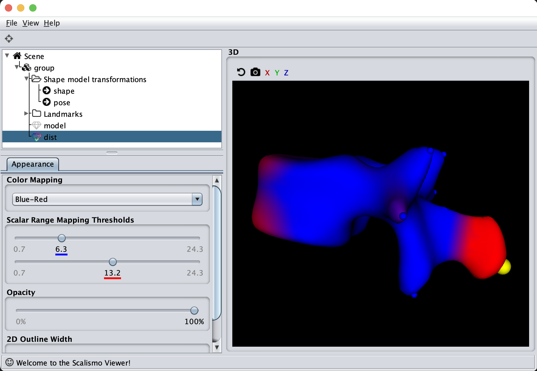
If we now instead use the created PCA model, we see that the kernel has incorporated that points on the mesh’s back side correlate with the selected landmark point. This is most likely connected with the size of the mesh.

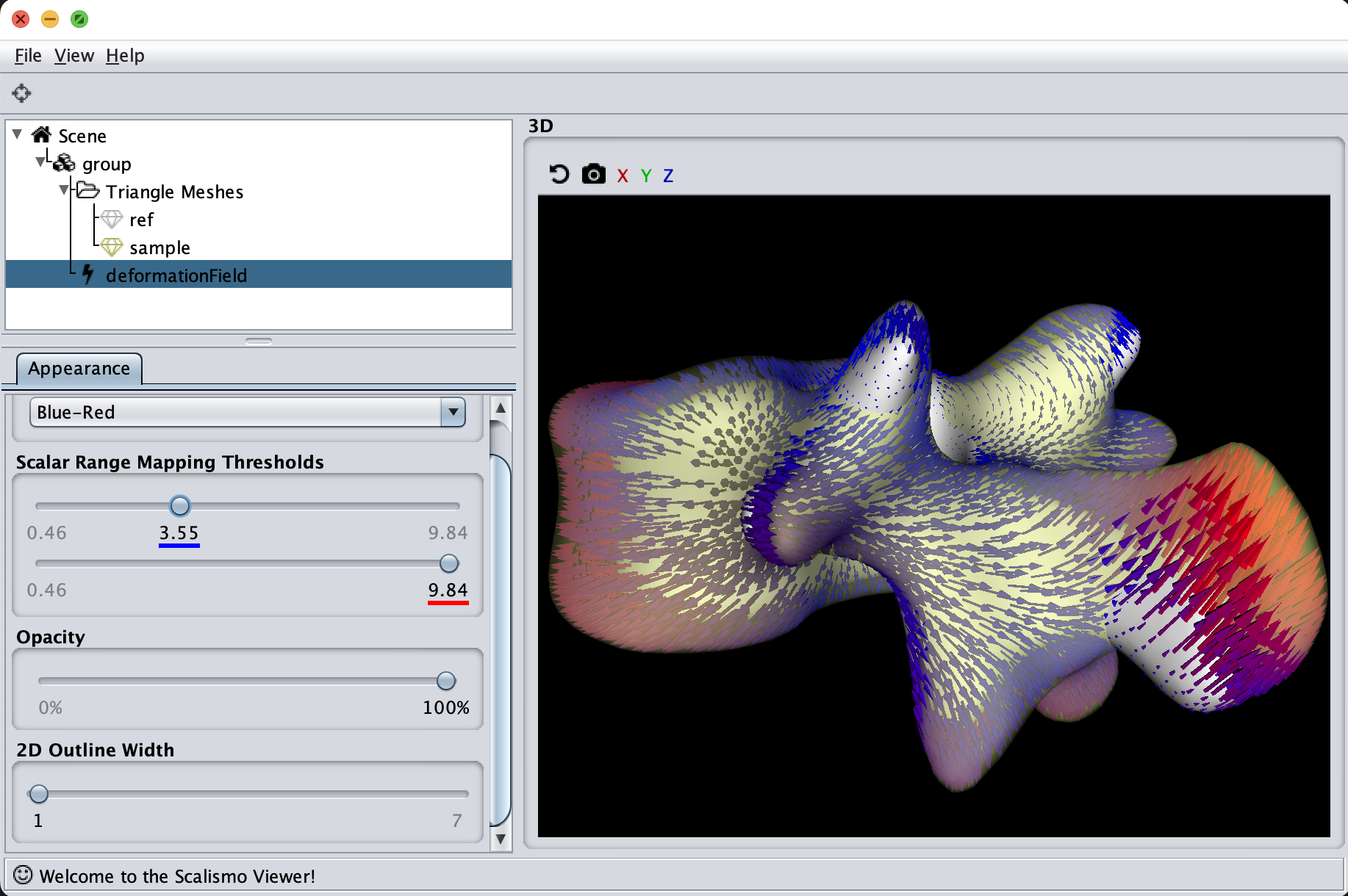
Deformation Fields

The last visualization method I want to show is how we can visualize deformation fields. This method is useful to check how smooth the deformation fields of a model are, as well as debugging correspondence estimation functions (such as ICP).

  val modelFile = new File(dataDir, "pca.h5.json")
  val model = StatisticalModelIO.readStatisticalMeshModel(modelFile).get 
  val ref = model.referenceMesh
  val sample = model.sample()

  val deformations = ref.pointSet.pointIds.map (id =>  sample.pointSet.point(id) - ref.pointSet.point(id)).toIndexedSeq
  val deformationField = DiscreteField3D(ref, deformations)

Summary

So, in summary, always visualize your models and try out different visualization methods to better understand the inner workings of your model.