How to Shape Model - Part 6 - Model evaluation

In this tutorial, I’ll go over different strategies to evaluate how good a shape model actually is.

This is the sixth tutorial in the series on how to create statistical shape models.

When it comes to model evaluation, nothing beats visual inspection of the models anatomical properties. With Scalismo-UI, we can inspect the individual principal components of the model one by one, as shown in the previous tutorials.

Load in the model and inspect the components. Then, try to randomly sample from the model to see if the shapes look realistic and anatomically plausible. And, very importantly, check that the model does not produce any kind of artifacts, such as self-intersection, inverted surface, or similar.

As a second step, consider the application where the model will be used and see if an automatic evaluation can be created. This could, for instance, be partial mesh completion. In such a case, you can synthetically remove parts of a mesh and check the model’s reconstruction with the ground truth. A good first step for this is to use the training data itself to begin with. For the training data, we know that the model should be able to represent it precisely. Then, after it is validated, we can move on to check the model’s performance on a test dataset where we also know the complete shape. And finally, the model can be used on partial data with no ground-truth data. This data can, of course, only be qualitatively evaluated.

Instead of comparing the complete meshes with a ground-truth mesh, another common evaluation strategy is landmark-based evaluation. Here, the model’s ability to identify specific landmark points is checked. For the model, we need to create a landmark file where the landmarks are placed on the template mesh. Then, we extract the position of the same point ID after fitting. The task is then to compare the landmarks with landmarks clicked manually by a human observer and possibly other automatic methods if available.

Model metrics

Besides qualitatively looking at the model or looking at the model performance on a specific application task, we can also look at some fundamental properties of the model, e.g.

1. If we randomly sample from the model, is the model only able to represent items from the dataset it was built? Or how different shapes is it able to create?
2. How good is the model in explaining items not in the training dataset?
3. How much variability does the model have, and how is this captured in the model?

These three properties are referred to as Specificity, Generalization, and Compactness. The metrics were introduced by Martin Styner in his 2003 paper: Evaluation of 3D correspondence methods for model building and has since become the standard when evaluating statistical shape models. Even though the methods provide good insight into a single model, the metrics are more useful when comparing different models, e.g., built on different datasets or built using different techniques.

The three metrics are usually reported by limiting the model to only use a certain number of the principal components. A 2D plot can then be created by plotting the number of principal components used on the X-axis and the metric value itself on the Y-axis.

Now, let’s go over our Vertebrae example and see how we can calculate each of the Metrics for the model.

Generalization

Generalization is measured on data items not in the dataset, so we will build our model on 7 of the Vertebrae samples and test on the remaining 3. A different strategy is to do the average of a leave-one-out calculation if limited data is available.

First, let’s define our training and test data items and build our model to be evaluated.

  val dataDir = new File("data/vertebrae/")
  val ref = MeshIO.readMesh(new File(dataDir, "ref_20.ply")).get
  val registeredDataFolder = new File(dataDir, "registered")

  val allPLYFiles = registeredDataFolder
    .listFiles()
    .filter(_.getName.endsWith(".ply"))
    .sorted
    .map(MeshIO.readMesh(_).get)

  val trainingData = allPLYFiles.take(7)
  val testData = allPLYFiles.drop(7)

  val dataCollectionTraining = DataCollection.fromTriangleMesh3DSequence(ref, trainingData)
  val dataCollectionTesting = DataCollection.fromTriangleMesh3DSequence(ref, testData)
  
  val ssm = PointDistributionModel.createUsingPCA(dataCollectionTraining)

Then, I’ll use Scalismo’s built-in ModelMetrics functionality to compute the model’s Generalization. To the function, we just need to pass the model and the data collection to be used for the calculation, in this case, our testing data.

  ModelMetrics.generalization(ssm, dataCollectionTesting).get

Let’s now call the function with the model limited to a certain number of principal components

  val generalization = (1 until ssm.rank).map(i => {
    val m = ssm.truncate(i)
    val g = ModelMetrics.generalization(m, dataCollectionTesting).get
    (i, g)
  })

Finally, let’s plot the output data

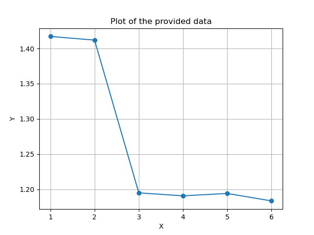
Note again that the X-axis specifies the number of principal components we use from the model, while the Y-axis is the average distance in millimeters between the model and the test meshes.

In the plot we see how the model Generalizes better the more principal components are used as would be expected.

If we compute the Generalization on the training data. When using all the principal components, the model should be able to precisely describe the data, i.e., a generalization of ~0.

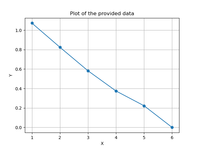
We also see that this is the case. This, again, can be used to check if there is a need for all the principal components in the model. If we, e.g., have a model with 100 principal components, but already after 50, it can perfectly describe both the training data and test data, this could hint towards some data not being needed in the model.

Specificity

For the specificity, we again use the function available in Scalismo’s ModelMetrics. To calculate the specificity value we pass in the training data, NOT the test data. We then specify a value describing the number of samples that the function should take. The higher this number is, the more precise the specificity number will be, but it will at the same time take longer to calculate. I usually use a value of at least 100. Internally, what is happening is that the function will produce 100 random samples from our model and then calculate the average distance between the sample and each item in the training data set. For the final specificity value, only the closest training data item is used. In other words, for each sample, the function finds the most similar item in the training data and calculates the average distance between the two. It then takes the average of all the 100 random samples that were produced.

  val specificity = (1 until ssm.rank).map(i => {
    val m = ssm.truncate(i)
    val s = ModelMetrics.specificity(m, trainingData.toSeq.toIterable, 100)
    (i, s)
  })

For the specificity, we should see that the more principal components that are used, we should be able to create shapes that are further away from the training data, i.e. a higher specificity value as also found in our case.

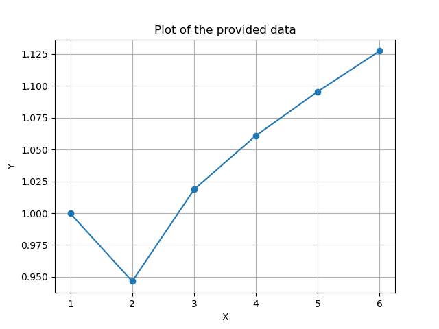
For specificity, the Axis’s describe the same as for Generalization - number of principal components and average distance in millimeters.

Compactness

Finally, the compactness is a measure the model’s ability to use a minimal set of parameters to represent the data variability. It is straightforward to calculate from the variance information stored about each principal component in the model.

  val compactness = (1 until ssm.rank).map(i => {
    val c = ssm.gp.variance.data.take(i).sum
    (i, c)
  })

We see that each added component adds a lot of new information to the model. Again, if we had a model with 100 principal components, we might see the values flatten out after some time, suggesting that the remining principal components provide little to no extra flexibility to the model.

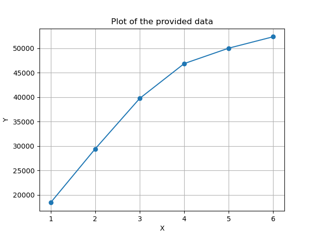
Also in this plot, the X-axis is the number of principal components that we use from the model, while the Y-axis is the total variance $mm^2$ in the model

While the model metrics can be used to evaluate individual models, they are more useful when comparing different models. As described, these models could be built from different datasets or using different techniques to create the model. Another useful area would be to compare the PCA model to different augmented models, as introduced in one of the previous tutorials. This can help to check if the model is augmented enough to generalize better but at the same time not too much to suddenly produce unrealistic shapes, i.e., high specificity.

Summary

So, in summary, always visualize your models and try to formulate an application-specific valuation for your model. Finally, I showed the commonly used metrics to evaluate statistical shape models: generalization, specificity, and compactness.

In the next tutorial, I’ll go over:

• Different ways to visualize statistical shape models.