How to Shape Model - Part 4 - Deformable template / Kernel design

In this tutorial, I’ll show you how to define the space of deformations our template mesh can undergo. So we will go from a static mesh, to a parameterized model that defines a space of deformations on the template, which we e.g. can randomly sample from to visually see the space of deformations.

Video walkthrough of the blogpost:

This is the fourth tutorial in the series on how to create statistical shape models. 

Defining the deformation space that the template can undergo might seem daunting with the endless possibilities of combinations.

Commonly asked questions on the Scalismo mailing list are “What parameters should I use for my model kernels” and “What kernels to choose”.

With a few heuristics in mind and a clear plan for defining your kernels, this task becomes a lot simpler.

For simplicity of this tutorial, I will not go into the formal definition of kernels. For this, I suggest you take a look at the tutorial from the scalismo tutorials from the Scalismo website or the instruction video from the statisticial shape modelling course at the University of Basel.

When talking about Gaussian Processes, a Kernel function describes how two data points are connected by describing their covariance. Simply said, when data point 1 moves, how much influence does this have on data point 2, if any at all? And also, how is the distance between point 1 and point 2 measured?

In this tutorial we will mainly look at the Gaussian kernel, and how we can modify it to, e.g. be symmetrical around a defined axis using the “symmetry kernel”, only be active in certain areas using the “Change Point Kernel”, or how to mix Gaussian kernels with different properties. Finally, I’ll show the PCA kernel, as introduced in the first video, and how we can make it more flexible by augmenting it with an analytically defined kernel.

5 different types:

1. Gaussian Kernel
2. Mixture of Gaussians
3. Symmetry Kernel
4. Changepoint Kernel
5. Augmenting a PCA kernel

Many more kernels exist than just the Gaussian kernel - but I often find mixing different Gaussian kernels sufficient, instead of using other kernel types.

For the Gaussian Kernel, we have two parameters to set:

1. The Sigma value defines the “width” of the kernel. The smaller this value is, the more local it is, meaning that only very close points will have a covariance over 0.
2. The scaling parameter. This can be used to adjust the “strength” or “amplitude” of the function.

val sigma = 100
val scaling = 1

val kernel = GaussianKernel3D(sigma, scaling)
val diagonal = DiagonalKernel3D(kernel, 3)

val gp = GaussianProcess3D[EuclideanVector[_3D]](diagonal)

One thing we need to remember when working with kernels is the dimensionality we work with. I will only show 3D examples, so it would also be possible to model the covariance between dimensions. But for simplicity, we always assume that the 3 dimensions are independent when analytically defining kernels. This is done using the DiagonalKernel.

With the kernel defined, we use it to define a Gaussian Process, which we’ll use later for regression purposes. The Gaussian Process that we have defined is continuous, but we are actually only interested in its values at the positions of our reference mesh. We can sample random deformations from the model:

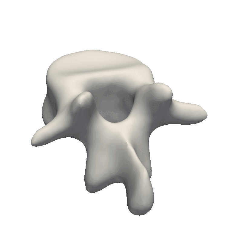
val ref = MeshIO.readMesh(new File("data/vertebrae/ref_20.ply")).get.operations.decimate(1000)
val sampleDeformation = gp.sampleAtPoints(ref)

val interpolatedSample = sampleDeformation.interpolate(TriangleMeshInterpolator3D())
// val interpolatedSample = sampleDeformation.interpolate(NearestNeighborInterpolator3D()) // Alternative interpolator
val sample = ref.transform((p : Point[_3D]) => p + interpolatedSample(p))

Internally, the sampleAtPoints create a huge covariance matrix. So depending on your memory, you might need to decimate the mesh first to get the code snippet to work.

We can get around the problem by approximating the covariance matrix instead of explicitly calculating it.

val lowRankGP = LowRankGaussianProcess.approximateGPCholesky(
  ref,
  gp,
  relativeTolerance = 0.1,
  interpolator = NearestNeighborInterpolator3D()
)
val sampleDeformation = lowRankGP.sample()
val sample = ref.transform((p : Point[_3D]) => p + sampleDeformation(p))

The relativeTolerance specifies the approximation error that is allowed. Setting it to 0.0 will mean that the low-rank approximation will precisely describe the full covariance matrix. Usually, a value around 0.01 is desired. But, to begin with, I often put a higher value like 0.5 or 0.1 to quickly calculate the function and visualize it. The interpolator to use very much depends on your application. Either the nearest neighbor or the triangle mesh interpolators are good choices to try out. And now with the low-rank function, we should be able to sample without having to decimate our reference mesh first.

A more convenient way to visualize samples from a Gaussian process is to build a Point Distribution Model from the low-rank Gaussian process. This allows us to directly sample meshes that follow the distribution represented by the Gaussian process and not have to deform the reference mesh manually from the given deformations.

val pdm = PointDistributionModel3D(ref, lowRankGP)
val sampleFromPdm : TriangleMesh[_3D] = pdm.sample()

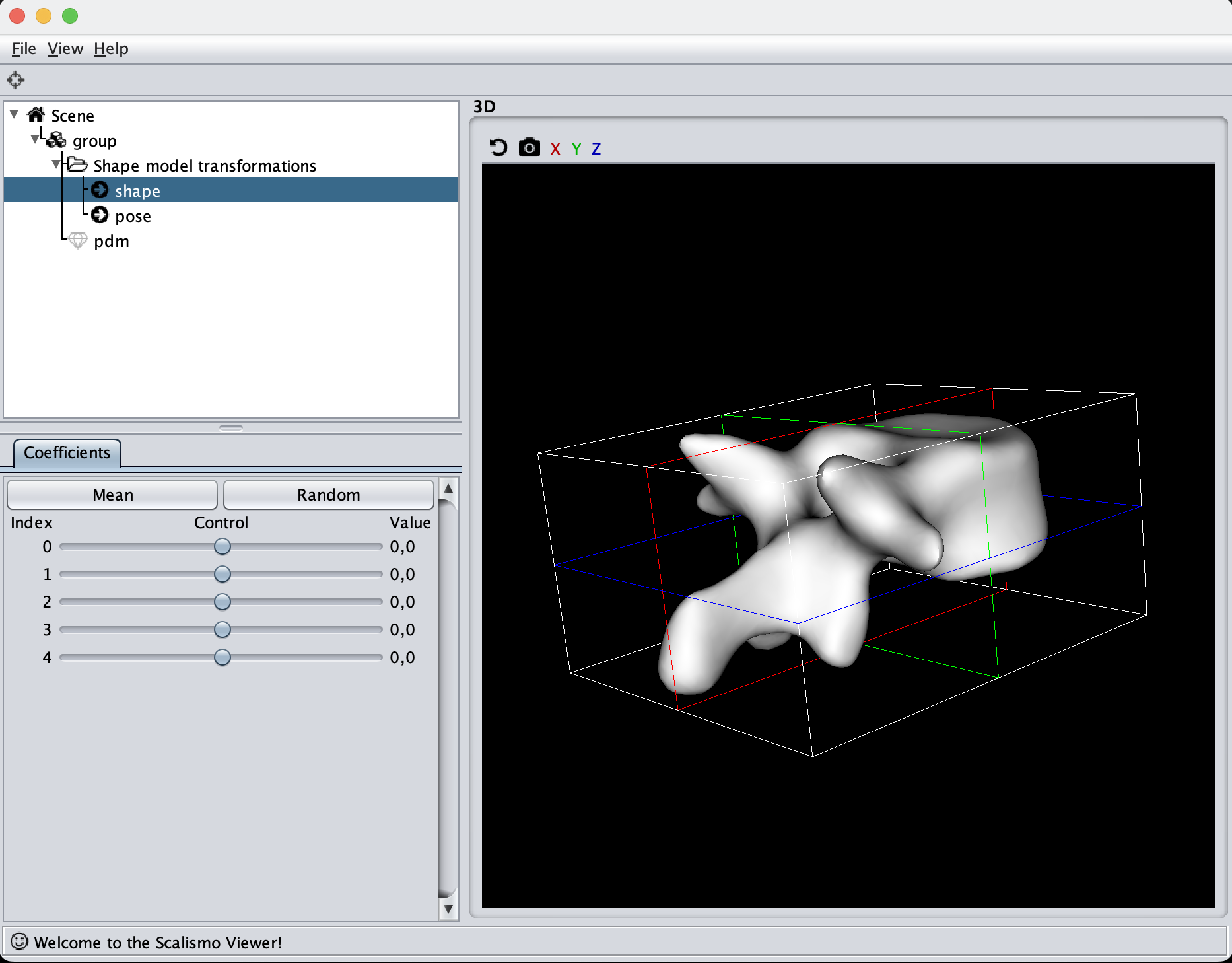
A Point distribution model can also be directly viewed in Scalismo, and we have access to all its parameters as well as a handle to sample from the model.

val ui = ScalismoUI()
ui.show(pdm, "pdm")

After having found the correct parameters to use for the model, it can be stored in a file and directly read again from disk, to avoid computing the model when we use it in the following tutorials.

StatismoIO.writeStatisticalTriangleMeshModel3D(pdm, new File("pdm.h5.json"))
val pdmRead = StatismoIO.readStatisticalTriangleMeshModel3D(new File("pdm.h5.json")).get

When inspecting the model, it is important to remember what the model will be used for. Our goal is to make the model flexible enough to represent all the other shapes in our dataset this also means that when we randomly sample from our model, it is perfectly fine that the deformations look exaggerated and produce non-natural shapes. The most important part is that the deformations are smooth such that the mesh does not intersect with itself. This also means that e.g. the mesh we see here is far from flexible enough to represent other meshes as it mainly shifts the position of the mesh around.

For the sigma value, I like to use a value that is 1/2 or 1/3 of the longest distance in the mesh. By looking at the scene view in Scalismo, we can get a feeling for the size of the mesh.

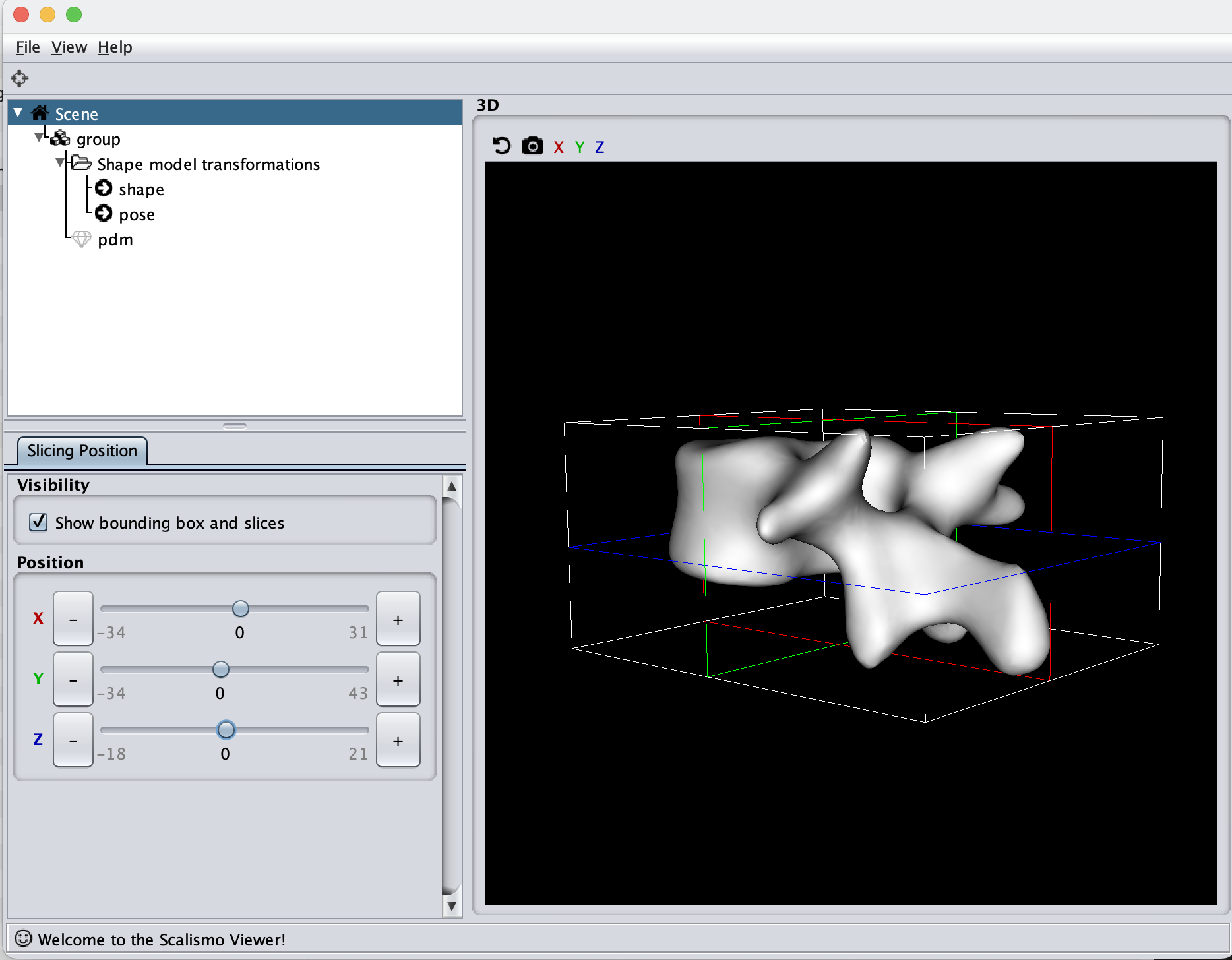
Here we see that the mesh is 65mm on the X-axis, 77mm on the Y-axis and 39mm on the Z-axis. With the current value of sigma to 100, this means that all points will have some correlation, what this ends up practically meaning is that the deformations will translate the mesh around. Let’s instead try to set Sigma to 35. Afterward, we can tune the scaling value if the magnitude of the deformations is not large enough.

I would recommend starting with a simple model like this with a simple Gaussian kernel and then only making it more advanced if needed.

And how do you know if more is needed? If the model has problems representing the meshes in your dataset, then more is needed. E.g. if some local curvatures are not nicely captured. You will only get to know so after running the non-rigid registration as introduced in the next two videos.

For completeness of this video, let’s continue adding some local deformations to our model by combining a kernel with a large sigma and one with a small sigma, I.e. a global and a local kernel. I typically visualize each model separately on the mesh and then combine the kernels afterward.

val kernelCoarse = GaussianKernel3D(35, 10)
val kernelFine = GaussianKernel3D(10, 3)
val kernel = kernelCoarse + kernelFine
val diagonal = DiagonalKernel3D(kernel, 3)

Symmetry Kernel

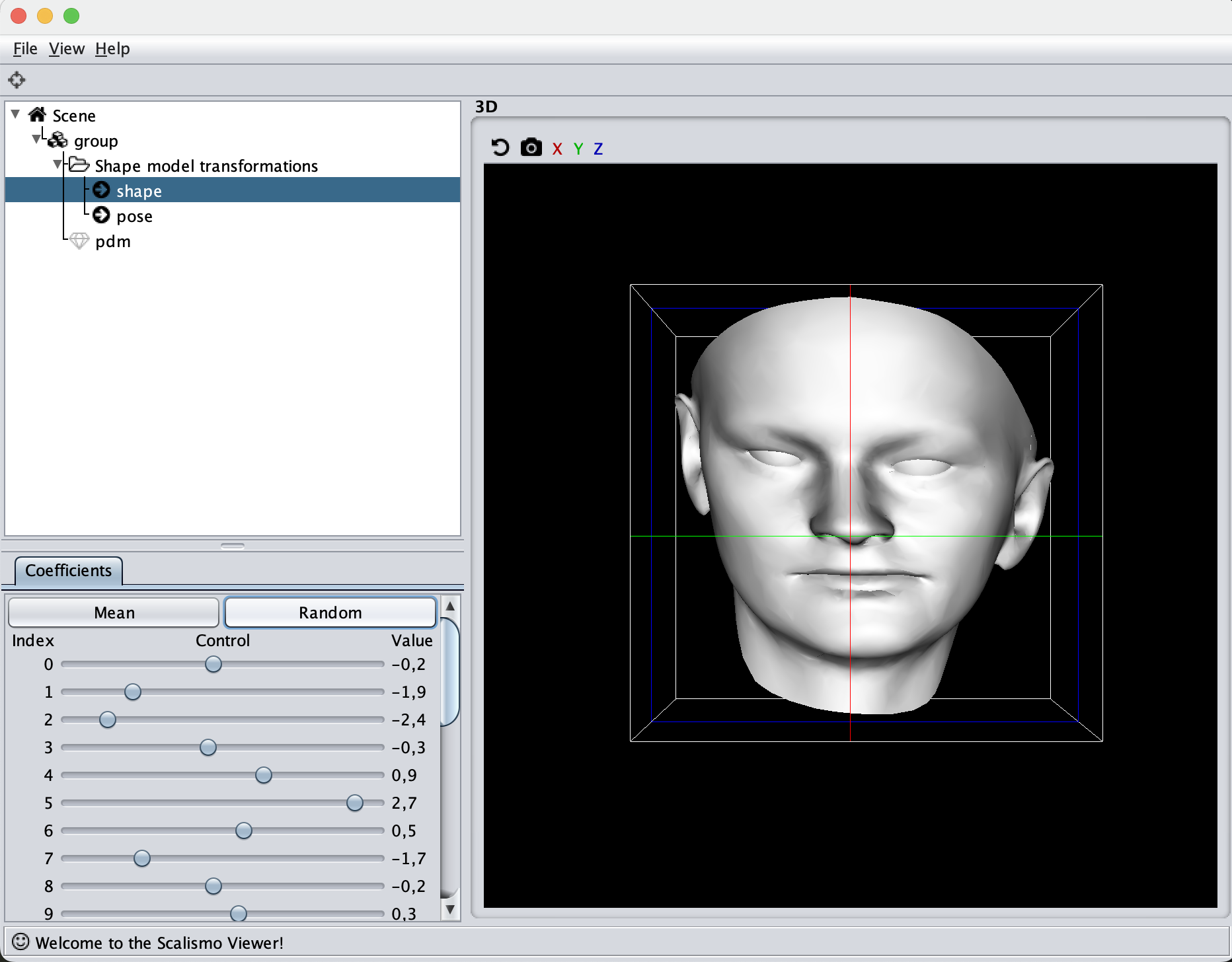
An alternative kernel is the symmetry kernel. To showcase this kernel, I’ll use the reference mesh from the Basel Face Model. First, let’s look at how a random sample from the face model looks like with the kernel

val kernel = GaussianKernel3D(100, 10)
val diagonal = DiagonalKernel3D(kernel, 3)

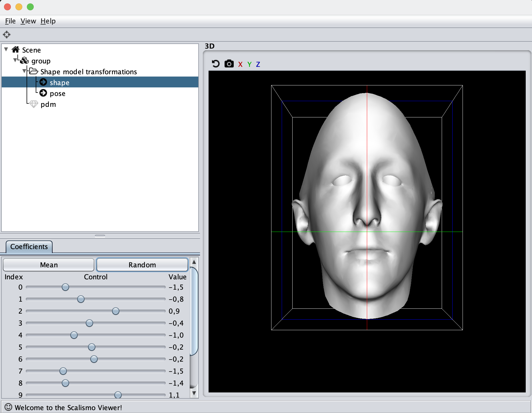
In the kernel, we’ll define the mesh to be symmetrical around the Z-axis. In reality, faces are of course not fully symmetrical, but it is a good global kernel to have, we can then always add local deformations to it.

case class xMirroredKernel(kernel : PDKernel[_3D]) extends PDKernel[_3D]:
  override def domain = kernel.domain
  override def k(x: Point[_3D], y: Point[_3D]) = kernel(Point(x(0) * -1.0 ,x(1), x(2)), y)

def symmetrizeKernel(kernel : PDKernel[_3D]) : MatrixValuedPDKernel[_3D] = 
  val xmirrored = xMirroredKernel(kernel)
  val k1 = DiagonalKernel3D(kernel, 3)
  val k2 = DiagonalKernel3D(xmirrored * -1f, xmirrored, xmirrored)
  k1 + k2

val diagonal = symmetrizeKernel(GaussianKernel3D(100, 10))

Changepoint Kernel

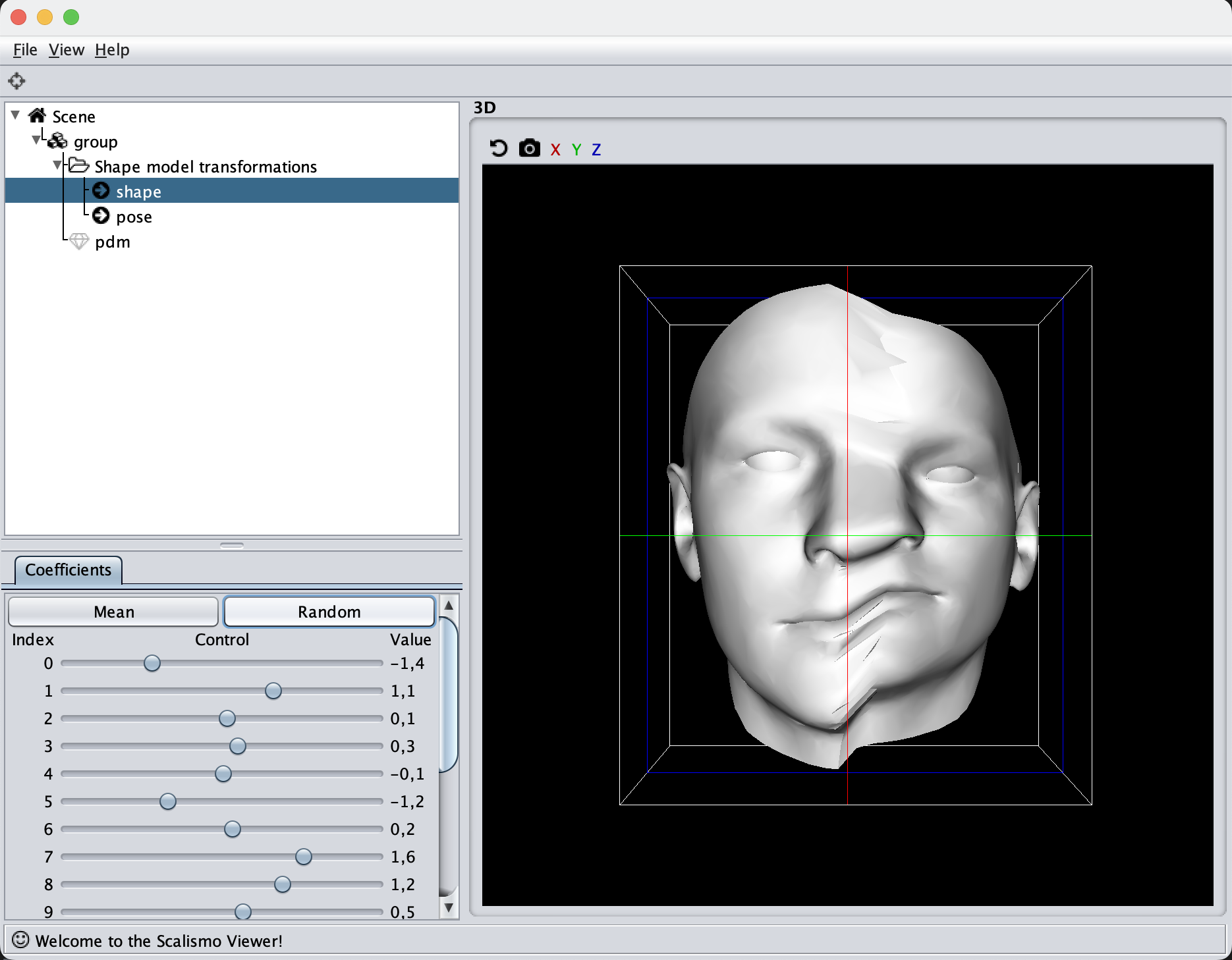
Another kernel is the change point kernel. For this, let’s stick with the face mesh and make one side of the face with one kind of kernel and the other side with an inactive kernel. In this way, we should see that only half of the face deforms when we sample from the model.

case class ChangePointKernel(kernel1 : MatrixValuedPDKernel[_3D], kernel2 : MatrixValuedPDKernel[_3D]) extends MatrixValuedPDKernel[_3D]():
  override def domain = EuclideanSpace[_3D]
  val outputDim = 3
  def s(p: Point[_3D]) =  1.0 / (1.0 + math.exp(-p(0)))
  def k(x: Point[_3D], y: Point[_3D]) = 
    val sx = s(x)
    val sy = s(y)
    kernel1(x,y) * sx * sy + kernel2(x,y) * (1-sx) * (1-sy)

val diagonal = ChangePointKernel(
  DiagonalKernel3D(GaussianKernel3D(100, 10), 3), 
  DiagonalKernel3D(GaussianKernel3D(1, 0), 3)
)

Make note of the s function, which defines which kernel to choose. This can either be binary to fully activate a kernel in a certain area, and fully deactivate it in others, or it can be made smooth as in the given example, such that the two kernels will have a smooth transition around the Z-axis in this case.

Augmented Statistical shape model

The final kernel I want to show is another mixture of kernels. This kernel could e.g. be used to iteratively include more data into your model. We start out with 10 meshes that are registered, from this, we can create a PCA kernel as also shown in the first video. Of course, 10 principal components rarely contain all small possible deformations, so we can augment the model e.g. with a Gaussian kernel, to make it more flexible.

val augmentedPDM = PointDistributionModel.augmentModel(pdm, lowRankGP)

And that’s the end of the practical guide to choosing your kernels and hyperparameters. Really the most crucial part is visualizing your models at every step of the way. Also, remember to look at the official Scalismo tutorial on Gaussian Processes and Kernels as the kernels are introduced there as well.

In the next tutorial I’ll show you:

• How to use the model we created to fit to a target mesh, also known as non-rigid registration.